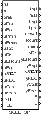
QCEDPOPT – Quadratic Cost Economic Dispatch Problem optimization block

Block SymbolLicensing group: ADVANCED

Function Description
The economic dispatch problem (EDP) with quadratic cost functions can be formulated as an optimization problem. Let’s have $n$ power sources (generators) with powers $P_{1}, P_{2}, \dots, P_{n}$ satisfying the constraints $P_{i, \min} \leq P_{i} \leq P_{i, \max}$ , $i = 1, \dots, n$ . Let the cost of the $P_{i}$ generation is given by the quadratic function $F_{i} = a_{i} P_{i}^{2} + b_{i} P_{i} + c_{i}, i = 1, \dots, n$ . Produce the given total power $P = P_{1} + P_{2} + \dots + P_{n}$ at the lowest possible price $F = F_{1} + F_{2} + \dots + F_{n}$ . The economic dispatch problem can be rewritten as

min F (P) = min \sum_{i = 1}^{n} (a_{i} P_{i}^{2} + b_{i} P_{i} + c_{i})

(15.1)

with respect to the equality constraint

P = \sum_{i = 1}^{n} P_{i}

(15.2)

and inequality constraints

P_{i, \min} \leq P_{i} \leq P_{i, \max}, i = 1, \dots, n .

(15.3)

The QCEDPOPT function block solves not only the economic dispatch problem (15.1) – (15.3) but much more complex problem. Let’s describe the extensions of this problem.

Very often it is not necessary to run all generators to achieve the power $P$ (connected to the input p of the block). If the $i$ -th generator is not running, it is assumed that the price of its zero power is zero. A given combination of running generators is feasible for the given power $P$ if $P$ is greater than or equal to the smallest of the minimum powers of the running generators and at the same time $P$ is less than or equal to the sum of the maximum powers of the running generators. Unfortunately, such combinations can be up to $2^{n}$ (e.g. if all minimum power of the generators is zero and $P$ is less than or equal to the smallest maximum power of all generators). In real applications, it is required that the given combination of generators be able to supply not only $P$ with a certain reserve (connected to the input pres), i.e. the sum of the powers of running generators must be at least p + pres. Minimum and maximum powers in (15.3) are elements of vectors referenced by inputs uPmin and uPmax.

This block calculates the price of all feasible combinations of generators, where the price coefficients in (15.1) are passed in the $n$ rows matrix referenced by uabc. Coefficients $a_{i}$ are in the first, $b_{i}$ in the second and $c_{i}$ in the third column of this matrix ( $i = 1, \dots, n$ ). If the $i$ -th generator is not running and should be started then this start can be evaluated by the starting costs (the generator is cold, some fuel is consumed for the start, etc.). Similarly, stopping a running generator can also be evaluated by stopping costs. Starting and stopping costs are optional and can be passed to the function block as fourth and fifth columns of the matrix referenced by uabc.

Quite often, in the short term, a higher total delivered power is required. This can lead to the start-up of other generators for only one or a few periods. Operating the generator for only a short time and then turning it off shortens the life of the generator. A similar situation occurs during a short-term decrease in the required power, when some generator is switched off for a short time. To eliminate these phenomenons, the so-called start horizon $n_{s}$ (input ns) is introduced in the QCEDPOPT block. The optimal EDP solution is not only sought for a given period, but over successive $n_{s}$ periods. In this case, the prediction of the required power is stored in a vector with at least $n_{s}$ elements which is referenced by the input uPns.

This problem is solved by the following algorithm:

For each step $k$ from $1$ to $n_{s}$ , calculate the optimal EDP solutions for all feasible combinations of generators (the number of these combinations can be up to $2^{n}$ ). This creates a state space with $n_{s}$ layers and a maximum number of elements $n_{s} \times 2^{n}$ .
Search the state space in depth. Start with a layer with index $i_{ns} = 0$ , which corresponds to the power prediction for the next period.
Go through the given layer from the index $i = 0$ (no generator runs) to $i = 2^{n} - 1$ (all $n$ generators run).
If the variant with index $i$ is feasible, save the value $i$ and go to the next step. If not, increment $i$ . If $i < 2^{n}$ then repeat this step, else go to step 7.
If $i_{ns} = n_{s} - 1$ , goto next step, otherwise increment $i_{ns}$ and go to step ?? (look for a feasible solution one layer deeper).
Here, we have a sequence of feasible solutions going through all $n_{s}$ layers. Calculate and store the cost function of this feasible sequence as sum of stored cost functions of particular solutions in each layer plus sum of (optional) starting and (optional) stopping costs between neighboring layers. Increment $i$ . If $i < 2^{n}$ then goto step 4
The end of the current layer $i_{ns}$ has been reached. Repeat: go one layer up ( $i_{ns} = i_{ns} - 1$ ) and restore the stored index $i$ for this layer until $i \geq 2^{n} - 1$ or $i_{ns} = 0$ . If $i_{ns} > 0$ , increment $i$ and go to step 4, otherwise the state space search is complete.

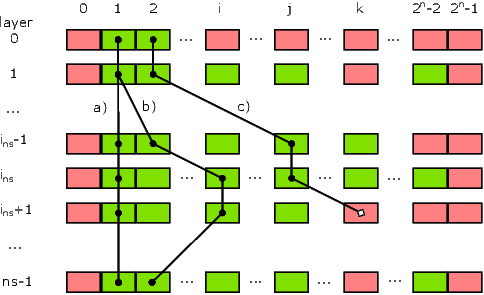
The following figure demonstrates the state space search in depth. Green rectangles corresponds to feasible state, red rectangles to infeasible states. Variants a) and b) represents feasible paths, path in variant c) is not feasible.

The number of all states of this algorithm in the state space grows exponentially. Ideally, the number of all feasible states is equal to

C_{f u l l} = {(2^{n})}^{n_{s}} .

(15.4)

Therefore, this algorithm is computable only for a low number of generators $n$ , (e.g. $n \leq 10$ ) and a short start horizon $n_{s}$ (e.g. $n_{s} \leq 10$ ). For a larger number of generators and/or a longer horizon $n_{s}$ , it is necessary to reduce the number of states in the state space. One option is to limit the maximum number of generator state changes (i.e. start a stopped generator or stop a started generator) at each step.

Assume that the state of just $m$ generators can be changed between two consecutive steps, which corresponds to the number of $m$ combinations of $n$ generators, i.e. $(\binom{n}{m})$ . If we allow a maximum of $m$ changes in each step, the number of variants for horizon $n_{s}$ is reduced to:

C_{r 1} = [\sum_{i = 0}^{m} (\binom{n}{i})]^{n_{s}} .

(15.5)

For small values of $m$ , which is very common in real cases, there is a significant reduction in the number of variants. The efficient implementation of this block’s algorithm is based on the calculation of internal fields for all combinations in one step. For the reduction just proposed, such a recalculation would have to occur each time the state of any generator changed, i.e. even during the search for an feasible path.

Therefore, it was finally decided to implement an even greater reduction in the number of states so that the maximum number of changes $m$ is not considered for adjacent steps, but over the entire horizon $n_{s}$ . In this case, a maximum of $n$ changes can occur in each of the $n_{s}$ steps. Of all such possibilities, we are only interested in those where $n \cdot n_{s}$ values change just $m$ times. For the maximum number of $m$ changes we receive

C_{r 2} = \sum_{i = 0}^{m} (\binom{n \cdot n_{s}}{i}) .

(15.6)

The maximum number of changes is specified in the parameter mchng. The above algorithm remains basically the same, only a reduced number of variants is tested. The original algorithm is used for the special value mchng = 0.

This block does not propagates the signal quality. More information can be found in the 1.4 section.

Input

ns	Starting horizon of power sources $↓$ 1 $↑$ 10	Long (I32)
p	Power to be distributed among sources $↓$ 0.0 $↑$ 1000000.0	Double (F64)
pres	Power reserve $↓$ 0.0 $↑$ 1000000.0	Double (F64)
uPns	Input reference to vector of distributed power prediction	Reference
uPact	Input reference to vector of powers of active (running) sources	Reference
uPmin	Input reference to vector of minimum powers of sources	Reference
uPmax	Input reference to vector of maximum powers of sources	Reference
uabc	Input reference to matrix of price coefficients	Reference
uDis	Input reference to integer vector of disabled reasons of sources	Reference
uEHours	Input reference to vector of engineering hours	Reference
uPopt	Input reference to allocated vector for optimum power distribution	Reference
uSTAT	Input reference to bool vector indicating running states	Reference
uREQ	Input reference to allocated bool vector for running requests	Reference
uCost	Input reference to optional vector for cost function values	Reference
uFeas	Input reference to optional byte vector for feasibility types	Reference
INIT	If TRUE then reinit optimization else optimize in real-time	Bool
HLD	Hold	Bool

Parameter

modesh	Starting heuristics mode $↓$ 0 $↑$ 3	Long (I32)
mchng	Maximum allowed number of run changes m per period $↓$ 0 $↑$ 10 $⊙$ 3	Long (I32)
nmax	Maximum value of n, nmax <= 10 $↓$ 0 $↑$ 10 $⊙$ 10	Long (I32)
nsmax	Maximum value of ns, nsmax <= 10 $↓$ 0 $↑$ 10 $⊙$ 10	Long (I32)
logflags	System log output flags $↓$ 0 $↑$ 63 $⊙$ 3	Long (I32)
ts	Sampling period. For ts = 0 the containing task sampling period is used $↓$ 0.0 $↑$ 1000000.0	Double (F64)
tspre	Time of power source prestart in seconds $↓$ 0.0 $↑$ 1000000.0	Double (F64)
svNF1	Substitute value in yCost for not feasible solution in the first step $⊙$ -1.0	Double (F64)
svNFns	Substitute value in yCost for not feasible solution in the whole horizon ns $⊙$ -1.0	Double (F64)

Output

fopt	Optimum value of cost function for horizon ns	Double (F64)
ifeas	Type of feasibility of the solution	Long (I32)
bopt	Bit combination of power sources to run for fopt	Long (I32)
bpre	Bit combination of power sources to be prestarted	Long (I32)
ncwc1	Worst case number of combinations depending on n power sources and parameter mchng	Long (I32)
lcount	Number of states traversed when searching the state space	Large (I64)
mem	Memory in bytes occupied by internally allocated working arrays	Long (I32)
yDis	Output reference to integer vector of disabled reasons of sources	Reference
yEHours	Output reference to vector of engineering hours	Reference
yPopt	Output reference to allocated vector for optimum power distribution	Reference
ySTAT	Output reference to bool vector indicating running states	Reference
yREQ	Output reference to allocated bool vector for running requests	Reference
yCost	Output reference to optional vector for cost function values	Reference
yFeas	Output reference to optional byte vector for feasibility types	Reference
E	Error indicator	Bool
iE	Error code	Long (I32)

[Back to top] [Up] [Next]